Reliability Diagrams for Probabilistic Forecast Evaluation

A probabilistic forecast earns trust only when its numbers mean what they say. The reliability diagram is the instrument that tests this, and reading it well separates rigorous evaluation from optimistic assumption. The sections below move from the definition of calibration to the construction and interpretation of these diagrams, and finally to the practical discipline their use demands.

What calibration means for a probabilistic forecast and why it is the right starting point

Calibration is the property that predicted probabilities match observed event frequencies across the full range of issued values. A forecast system is calibrated when, among all cases where it issued a probability near 0.80, the event occurred about 80 percent of the time. This standard is distinct from accuracy and is not implied by it. A model can be correct in most of its classifications while remaining profoundly miscalibrated in the confidence it attaches to those classifications.

The literature uses two terms for the same property: calibration and reliability. The interchangeability matters because a reader who encounters one term in meteorology and the other in machine learning may not immediately recognize that they refer to the same standard. Establishing this equivalence early removes a persistent source of confusion.

Calibration matters because forecast probabilities, uncertainties, and expected values must be interpretable at face value in decision-making contexts. When a forecaster issues a probability of precipitation, a calibrated system permits the recipient to treat that number as a statement about the world: under comparable conditions, this event will occur at the stated frequency. Miscalibrated confidence steers decisions wrong even when a model's raw accuracy is high, because the user acts on a probability that does not correspond to any real frequency. The property is necessary, not optional, if probabilities are to be used in quantitative decision-making. A probability that is not calibrated is not a valid input to expected-value calculations, threshold-based triggers, or resource-allocation rules.

What a reliability diagram is and how to read it

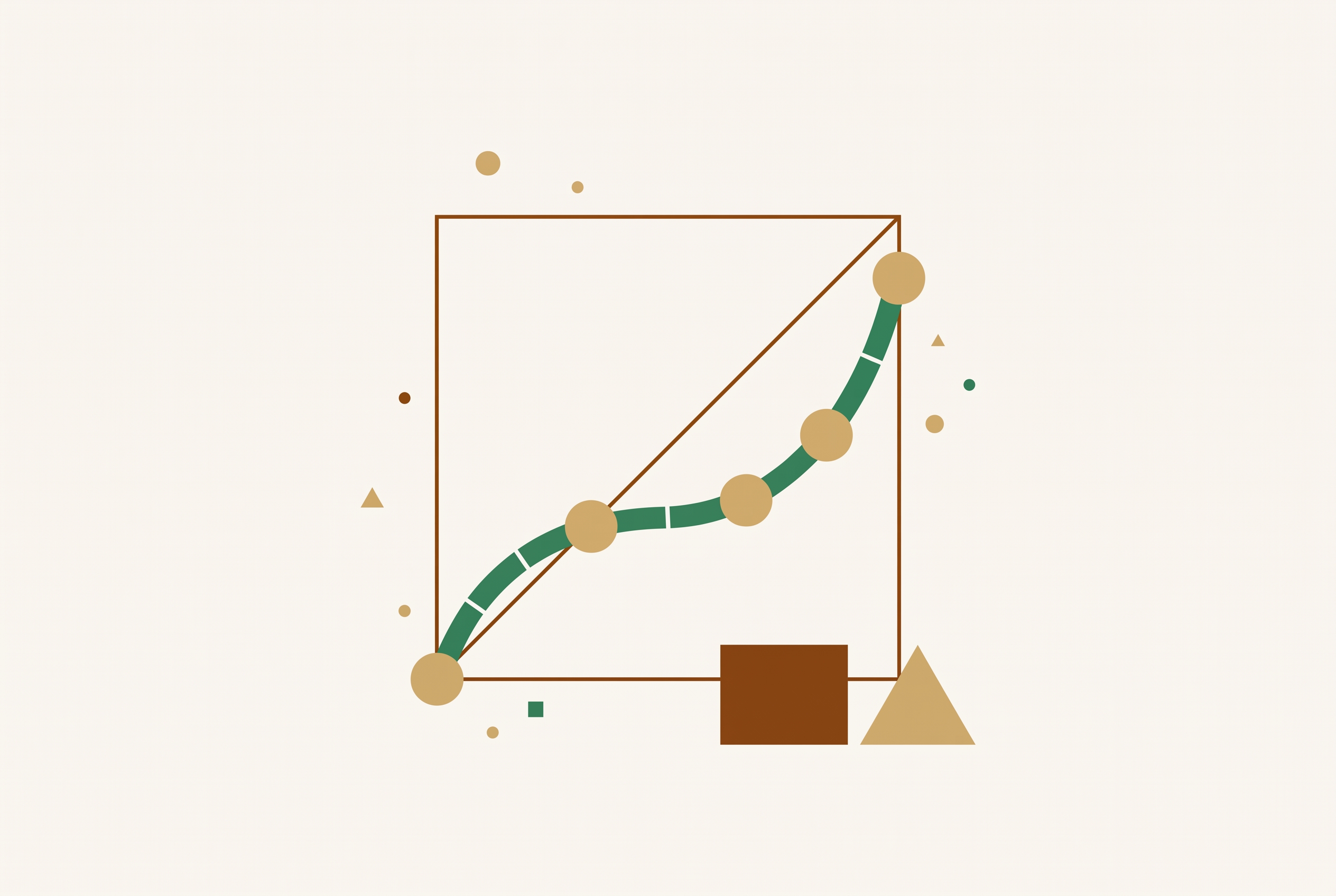
The reliability diagram is the standard visual test of calibration. It plots observed event frequency against predicted probability, and a forecast is calibrated when the plotted curve lies close to the diagonal. The diagonal is not an aspiration. It is the definition made visible.

Reading the diagram requires attention to where points fall relative to the diagonal. Points on or near the line indicate calibration. Points below the diagonal indicate overconfidence: the forecast issued probabilities more extreme than the empirical frequencies that followed. Points above the diagonal indicate underconfidence: the forecasts were too conservative. The direction of departure carries diagnostic information about the nature of the miscalibration.

A diagram can display more than the calibration curve. A no-skill line marks the region where the forecast adds no value over climatology, and regions of positive and negative Brier Skill Score identify where the forecast improves on or falls short of that baseline. A sharpness histogram, typically shown as a secondary panel, records how often each probability level is issued. The calibration curve and the sharpness histogram together reveal whether a forecast is also informative, not merely unbiased. Overforecasting in raw grid-point precipitation forecasts, for example, appears as a pronounced departure below the diagonal at non-trivial probability levels, with almost no significant performance above the no-skill line.

The tool originated in meteorology and has become central to machine learning. The migration was driven by the recognition that modern neural networks are uncalibrated, unlike those from a decade ago. A reliability diagram makes that deficiency visible in a single image.

Why the classical binning approach produces unstable diagrams

The classical method of constructing a reliability diagram divides forecast probabilities into fixed bins and plots the mean forecast probability against the observed frequency within each bin. The approach is intuitive, but it is highly sensitive to the choice of bins. The visual appearance can change drastically under the slightest adjustment.

A concrete demonstration makes the problem plain. Choices of 9, 10, or 11 equidistant bins for an EMOS forecast at Niamey, Niger yield drastically distinct reliability diagrams from the same underlying data. Three defensible bin counts produce three different visual stories about the same forecast system. The instability is not a minor cosmetic issue: the bin choice is typically arbitrary, not theoretically justified, and similar instabilities affect numerical calibration measures such as the Brier score reliability component. A practitioner who changes the bin count and sees the miscalibration vanish has not fixed the forecast. The diagnostic has simply shifted. The problem persisted despite well-argued calls for reproducibility and stability. Researchers across disciplines continued to use ad hoc bin choices, and the gap in practice was precisely what the CORP approach was designed to close.

How the CORP approach resolves the binning problem

The CORP approach generates provably statistically consistent, optimally binned, and reproducible reliability diagrams in an automated way. It removes the need for arbitrary bin choices, which means the instability that plagued the classical method disappears by construction rather than by convention. The mechanism is nonparametric isotonic regression implemented via the pool-adjacent-violators algorithm, known as PAV. The CORP reliability diagram shows the graph of PAV-recalibrated forecast probabilities. Rather than imposing a bin structure on the data, the algorithm finds the monotone curve that best fits the observed frequencies, and the diagram displays that curve directly.

CORP adds more than a stable plot. It produces a numerical measure of miscalibration, abbreviated MCB, that quantifies how far the forecast departs from calibration. It also yields a score decomposition expressing the mean Brier score in terms of three components: miscalibration (MCB), discrimination (DSC), and uncertainty (UNC). The decomposition generalizes to any proper scoring rule, which means the same analytical structure applies beyond the Brier score. An applied demonstration shows the value of the approach: CORP reliability diagrams for probability-of-precipitation forecasts at Niamey compare ECMWF's ENS, statistical logistic models, and another deep-learning model on a single diagram with full score decomposition.

The framework has since been extended beyond binary events. Gneiting and Resin generalized it to threshold, mean, and quantile reliability diagrams for continuous outcomes. They treat traditional unconditional calibration notions as weak special cases and recommend that priority be given to probabilistic and marginal calibration checks. The extension means the same principled construction applies across the full range of forecast types.

A hidden trap in ensemble forecasts: slope attenuation from finite ensemble size

Even a perfectly reliable ensemble will produce attenuated, flattened slopes in conditional reliability diagnostics when ensemble size is finite. The reason is that finite-ensemble sampling noise biases the estimated relationship between forecast probabilities and observed frequencies. The effect can be mistaken for genuine miscalibration, and the mistake is consequential: a forecaster may conclude that a system is deficient when the apparent deficiency is an artifact of ensemble size. Richardson established in 2001 that this manifests as a clockwise tilt in standard reliability diagrams, a flattening of the slope relating observed event frequency to forecast probability. The finding is not new, but its practical implications remain underappreciated.

The framework from Spaeth and Roberts builds on this foundation. It derives analytical expressions for the expected slope attenuation and proposes practical estimators computable directly from ensemble data, without reference to observational data. The effect is illustrated using ECMWF 2-metre temperature sub-seasonal ensemble forecasts, where finite-ensemble slope attenuation substantially affects both the spread-error relationship and tercile-based reliability diagrams. The practical implication is direct: attenuated conditional slopes should not be interpreted as evidence of forecast deficiencies unless finite-ensemble effects have been explicitly accounted for. The benchmark for evaluation can now be adjusted for this effect, and the adjustment should be made before any judgment about forecast quality is reached. The diagram remains the right instrument. It simply requires informed interpretation.

What reliability diagrams reveal across different forecasting domains

Reliability diagrams expose characteristic patterns of miscalibration that differ by model type and domain, and those patterns point directly to the source and nature of the problem. The same tool applied across contexts surfaces distinct failure modes that would otherwise remain hidden. In heavy precipitation forecasting, the Radar Maxima product from DWD, built on the ICON-D2-EPS ensemble system, offers a clear case. Point-based forecasts yielded low probabilities for extreme events due to spatial displacement errors. Area-based aggregation within 40 km neighbourhoods improved reliability and sharpness over the point-based approach. The diagram made the improvement measurable. The practical frequency that motivated the product is striking: radar detects events with more than 25 mm/h within a 40 km radius approximately once every 4.25 months.

In image classification, the pattern runs in an unexpected direction. Reliability diagrams for current-generation models, ConvNeXt, EVA, and BEiT, and traditional models, Swin Transformer, ViT, and ResNet, on ImageNet reveal that despite superior classification performance, current-generation models exhibit systematic underconfidence. They underestimate their own predictive confidence. This is a reversal of the overconfidence pattern typical of older models, and it means the newer models leave useful probability mass on the table even as they classify more accurately.

In brain-inspired training, reliability diagrams exposed a bias present before learning began. Conventionally initialized networks exhibited overconfidence and class bias before training even started. A random-noise warm-up procedure mitigated this initial bias and calibrated confidence to close to the chance level. The diagram functioned as a diagnostic of initialization, not merely of the trained model.

Where standard calibration checks stop short: the case of tail events

A forecast can satisfy standard notions of calibration and still issue unreliable probabilities for extreme events. Allen et al. demonstrate this gap by introducing the notion of tail calibration, which is a stricter requirement than the calibration standard captured by a conventional reliability diagram. The gap matters because extreme events typically lead to the largest impacts on forecast users. A calibration check that does not interrogate the tails can give false confidence precisely where confidence is most consequential. A system may look well calibrated across the bulk of its issued probabilities while remaining systematically wrong about the rare events that carry the most weight in decision-making.

A proposed remedy moves tail calibration from diagnostic to objective. A June 2025 arXiv preprint proposes loss functions based on weighted proper scoring rules that enforce tail calibration during training. The approach places calibration into the training objective itself, rather than treating it as a post-hoc check. The trade-off is real: practitioners must choose the weight function, which adds new degrees of freedom, and there is no settled consensus on a universal approach. For high-impact forecasting applications, a standard reliability diagram alone is not enough. It remains indispensable, but it must be supplemented with tail-specific diagnostics.

Open questions in how to summarize calibration as a single number

There is no settled consensus on the best scalar measure of miscalibration to accompany a reliability diagram. The diagram shows where and how a forecast departs from calibration, but a single number is often needed for comparison across systems, and the choice of that number remains a live methodological question. The competing approaches are clear. Expected Calibration Error, or ECE, is the histogram-based scalar most widely used in machine learning. It is easy to compute and easy to report, but it inherits the binning sensitivity of classical diagrams. The same instability that made classical reliability diagrams unreliable transfers to ECE when bin choices shift.

The CORP-based MCB takes a different path. It is derived automatically from the PAV algorithm, which avoids ad hoc binning entirely, and it connects directly to the Brier score decomposition. The practitioner faces a real choice between convenience and principled construction, and the literature does not yet provide an authoritative default. New tooling reduces the implementation friction without resolving the underlying conceptual debate. Fan et al. introduced Calzone, a Python package providing reliability diagrams with error bars, class-conditional calibration error, different binning schemes, and statistical significance testing for miscalibration. The package makes it easier to run the analysis, but the choice of scalar remains the analyst's to make and defend. Awareness of this open question is itself part of rigorous evaluation.

How to apply reliability diagrams rigorously in practice

Rigorous use of reliability diagrams requires attending simultaneously to construction method, ensemble-size effects, sharpness, and the tail. No single check is sufficient on its own. The following discipline synthesizes the caveats and advances from the preceding sections into a coherent workflow.

First, prefer the CORP and PAV-based approach over fixed-bin diagrams. This avoids instability under arbitrary bin choices and ensures that the diagram shown is reproducible by others. Use the accompanying MCB-DSC-UNC decomposition to identify whether a miscalibration problem is primarily one of reliability, discrimination, or inherent uncertainty. The decomposition tells the practitioner where to direct effort, rather than merely that something is wrong. Add error bars or uncertainty bands, available via resampling or asymptotic theory in CORP and in tools such as Calzone, to distinguish genuine miscalibration from sampling noise.

Second, correct for ensemble-size effects. When working with ensemble forecasts of finite size, compute the expected slope attenuation and adjust the benchmark before judging whether an attenuated slope reflects a real forecast deficiency. Skipping this step leads to false conclusions about forecast quality, particularly for smaller ensembles.

Third, always read the diagram alongside a sharpness histogram. A calibrated but uninformative forecast is a distinct failure mode from miscalibration. A forecast that always issues the climatological probability is perfectly calibrated and entirely useless. The sharpness histogram exposes this. Fourth, for high-impact applications, supplement the standard diagram with exceedance-event reliability diagrams and quantile hit-rate diagnostics to assess tail calibration separately. For continuous outcomes, extend beyond binary reliability diagrams to threshold, mean, and quantile reliability diagrams using the framework of Gneiting and Resin, treating probabilistic and marginal calibration checks as the priority.

The reliability diagram is not a single plot but a family of complementary diagnostics. Construction method, uncertainty quantification, ensemble-size correction, sharpness, and tail behavior together give a complete picture of calibration. A practitioner who attends to all of them earns the right to trust the probabilities a forecast issues.